Things I Wish I’d Known Prior to Creating a Queuing System
A project that I am currently working on implements a distributed data processing system. It entails the following phases: first, a number of machines simultaneously generate certain messages, these messages are subsequently queued, three streams fetch messages from the queue, and after final processing, they are uploaded to the Redis database. There’s also a crucial time limit – no more than 4 seconds should elapse between the message “inception” in the message-generating computer and the upload of the processed data to the database in 90% of the cases.
At a certain point, it became clear that we were not complying with this requirement despite all the invested efforts. Several measurements and a short foray into the queuing theory have led me to conclusions which I would like to have communicated to myself several months ago, when the project was just getting underway. I can’t send a letter to the past, but I can write an article that may relieve someone who’s just deliberating queue usage in their system of some troubles.
I started with measuring the time spent by the message in various processing phases, and obtained the following approximate results (in seconds):
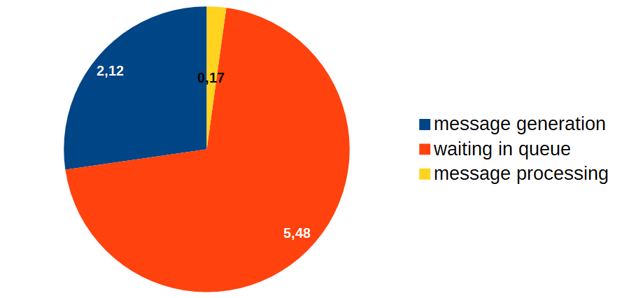
Thus, despite the fact that message processing takes up a rather small time period, it spends the most time in the queue. How is that possible? And the main issue is: what’s the way to combat it? If the image above was the result of regular code profiling, it would be apparent: the procedure marked in red should be optimized. But the trouble is that in our case nothing happens in the red zone, the message is simply queued! It’s clear that message processing requires optimization (the yellow part of the diagram), but several questions emerge – how will this optimization affect the length of the queue and what are the guarantees that we will even be able to attain the desired result?
I recalled that queuing theory deals with queue waiting probability estimates. We have not, however, covered this material at the university, so I was about to immerse in Wikipedia, PlanetMath and online lectures, which, just like the horn of plenty, showered me with an abundance of information on Kendall’s notation, Little’s law, Erlang’s distribution, et cetera.
The analytical results of queuing theory abound in rather rigorous math, and the majority of these results were obtained in the 20th century. Studying this matter is captivating, albeit rather long and laborious. I cannot claim that I was able to immerse myself deeply in the subject.
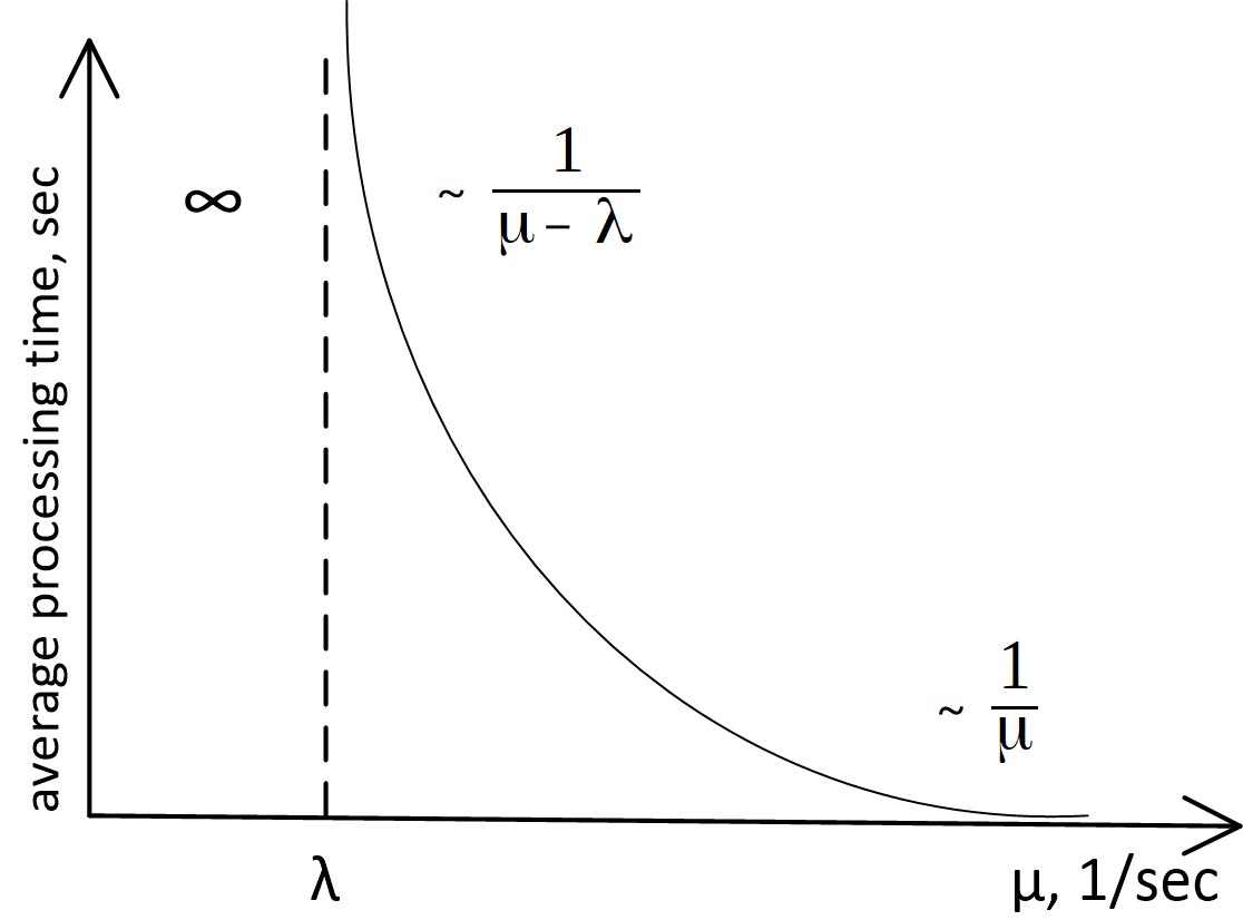
However, even after merely skimming the surface of queuing theory, I discovered that the main conclusions applicable in our case are self-evident, their substantiation requires mere common sense, and they may be depicted on a graph of queuing system processing time as a function of the server throughput rate, as follows:
Here
-
— server throughput rate (in messages per second)
-
— average frequency of incoming requests (in messages per second)
-
Average message processing time is intercepted on the ordinate.
The precise analytical form of this graph is the queuing theory’s subject of study, and for queues M/M/1, M/D/1, M/D/c, etc. (if you don’t know what this means, see Kendall’s notation) this curve is described by very different formulas. However, whichever model is used to describe the queue, the external appearance and the asymptotic behavior of this function will be the same. It’s possible to prove it by simple reasoning, so let’s get to that.
Let’s start by looking at the left side of the graph. It’s entirely clear that the system won’t be stable if (throughput rate) is less than (input frequency) — the messages arrive for processing at a greater frequency rate than we can process them, the queue grows indefinitely, and we’re in serious trouble. Basically, the case is always abnormal.
The rather simple fact that in its right part the graph asymptotically approaches does not require an in-depth analysis for proof. If the server functions extremely fast, and there is practically no waiting in queue, the total time spent in the system is equal to the time it takes the server to process a message, which equals precisely .
The only fact that may not seem apparent at first is that as approaches on the right side, the time of waiting in queue increases to infinity. In fact, if , it means that the average message processing rate is equal to the average message input rate, and it intuitively seems that in this setup the system should be able to handle it. Why does the graph of time as a function of server productivity at point fly out into infinity, instead of behaving in the following manner?
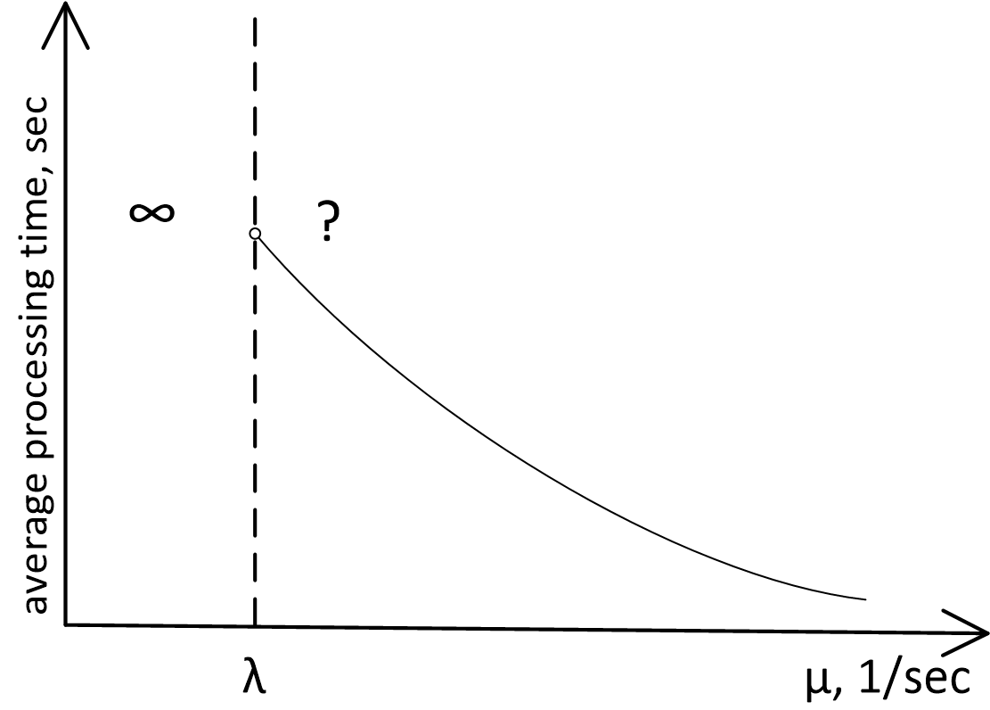
However, this fact can be established without in-depth mathematical analysis! For this purpose, one needs to understand that the server may exist in two modes as it processes messages: 1) busy, or 2) idle, when all requests have been processed, and no new ones have arrived in the queue.
The tasks arrive in the queue at an uneven rate, by fits and starts — the number of events per unit of time is a random value, described by the so-called Poisson distribution. If, during a certain time interval, the tasks come in infrequently and the server is idle, it cannot “save” the time during which it was idle and use it for processing of subsequent messages.
This is the reason why the average event output time will always be lower than the peak server throughput rate.
In turn, if the average output time is lower than the average input time, it leads to an infinite increase in the average queue waiting time. For queues with Poisson distribution at input and a consistent or exponential processing time, the waiting time at saturation point is proportional to
Conclusions
Thus, as we examine our graph, the following conclusions emerge:
-
The time of message processing in a queuing system is a function of the server throughput rate ( ) and the average incoming message arrival rate ( ), and, to put it even simpler, it’s a function of the ratio of these values ( ).
-
When designing a queuing system, you need to evaluate the average incoming message arrival rate ( ) and include the server throughput rate
-
Any queuing system is dependent on the ratio between and , and may exist in one of the three modes:
-
Abnormal mode — . The queue and the system processing time are increased indefinitely.
-
Near-saturation mode: , but not significantly. In this case, even slight alterations of the server throughput rate affect the system productivity parameters significantly in both directions. The server requires optimization! Meanwhile, even slight optimization may prove extremely beneficial for the entire system. The evaluation of the message arrival rate and our server’s throughput rate have demonstrated that our system had been functioning precisely near the "saturation point."
-
“Negligible queue waiting time” mode: . Total time in the system approximately equals the time required for processing by the server. The need to optimize the server is determined by external factors, such as the share of the queuing subsystem in the total processing time.
-
Having grappled with these issues, I started to optimize the event processor. This is how things have shaped up in the end:
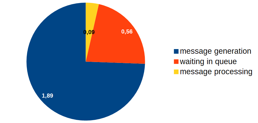
Alright, now let’s optimize the message generation time!