Hidden Complexity of a Routine Task: Presenting Table Data in User Interface
This article is a condensed recap of my presentation made at the JPoint conference.
Introduction: Problem Statement
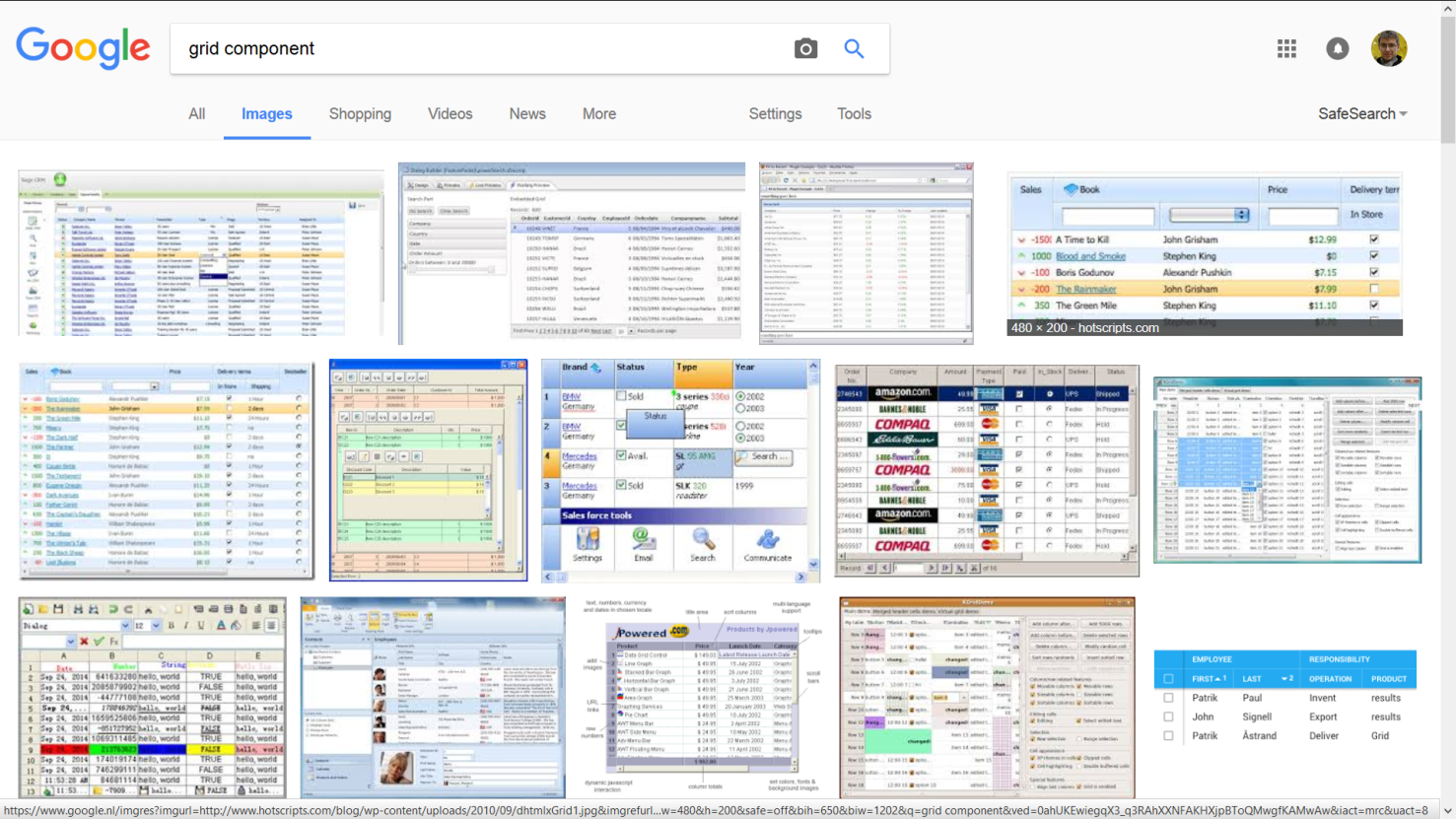
The grid component is one of the most commonly used user interface elements. All of us see it numerous times a day. The grid is the most appropriate representation of relational database tables since it illustrates our understanding of how rows and columns of data are stored in a database.
The grid component is so common that it may seem that well-known methods of its implementation have been found long ago. But if you start to go deeper, it turns out that there’s nothing simple about the task of displaying tabular data, and that there’s no universal solution to it.
In this article, I will discuss the task of displaying tabular data, I will demonstrate the shortcomings of some "naive" approaches to its solution, and then I’ll digress to the mathematical and algorithmic jungles where the attempt to generalize the solution of this problem leads us.
Grid Component Requirements
The grid component has two main functions.
-
Scrolling gives the user an illusion of working with a huge "sheet," which displays all the available data from the table. The user can view any part of this "sheet" by moving the vertical scroll bar knob.
-
Positioning. If we know the primary key value for a certain entry, we should be able to locate this entry in the grid (with adjoining entries appearing and the vertical scroll bar knob positioned to the right place).
Non-functional requirements are as follows:
-
The grid must work quickly, that is, it shouldn’t overload the database with its requests, since there may be a lot of users.
-
The grid must be convenient, that is, it should allow users to browse the data in a way they want.
-
It is also desirable for the speed and convenience not to decrease with the increase in the number of entries, so that, working with the grid should be equally fast and convenient whether there are only ten entries or a million.
Simple Approaches to Solving the Problem of Grid Construction
#1: Reading Data into an Array
The first thought that comes to mind is — if the grid is a virtual "sheet," a two-dimensional array, then in order to display the data it’s enough to read this data from the database into an in-memory array. Imagine that we’ve succeeded, and the entire table is stored as an array.
The good news is that if we have really succeeded, then we have, in fact, solved the problem. Since the purpose of scrolling comes down to selecting entries from to , where is the number of entries that visually fit the screen in the grid. This operation comes down to operations of accessing an array element by index, and this operation is known to be very fast with O(1) complexity.
How is positioning conducted? Assuming that the entries are ordered by a set of columns (an assumption that can be always considered true), then we can arrange a binary search and accomplish the positioning just as quickly, in O(log (N)) time (where N is a total number of entries).
It turns out that reading all the data into an array solves the task of displaying the grid. Moreover, when we can indulge ourselves and do it, nothing should be done differently.
The bad news is that the initial data loading into the array has O(N) complexity. The amount of data in the system grows every day, increasingly more entries have to be downloaded to the grid, and the user has to wait increasingly longer for the grid to open. At best, the user is shown a progress bar at this point, at worst — the user just waits longer and longer until the application unfreezes.
An additional problem is that the data in the database are not immutable, they are constantly changing with time. Therefore, in order not to have obsolete data the user must periodically update the grid, clicking the refresh button again and again and waiting for the download. It is best to avoid this.
#2: Request Only the Necessary Data From the DB Using OFFSET
Let’s try to consider the problem from a different side. Why download all the rows of the table, if the user will read only several dozen of them at most? You can try using the RDBMS tools to extract only the rows to be displayed.
Let’s start with the good news. Half of the positioning problem is resolved trivially. Let’s say we need to locate a record with the key k in the grid and display it along with the records closest to it. You can do this using a query of the type
SELECT … WHERE k >= … LIMIT …where the value of the LIMIT parameter is the number of records that fit on one screen.
If there is an index over the k field, such a query will work very fast, and we’ll immediately get the range of records that we need.
This, however, is where the good news ends. Because after displaying the required record, we also need to set the scroll bar to the desired position. To do this, we need to calculate the number of records that are less than this key, that is, to perform the COUNT operation.
COUNT is a long-running and expensive operation; its execution time increases as the number of records in the table grows.
When working with a grid, we often use scrolling rather than positioning. What does the selection of records, starting with the nth one, entail for the database? Most modern databases support the OFFSET keyword for this purpose. If we need to select records in a certain query, starting, say, with one-hundred-thousandth, then we will write
SELECT … FROM … OFFSET 100 000Just as COUNT, OFFSET is an expensive operation. For example, in the PostgreSQL documentation, the following clarification is made: “The rows skipped by an OFFSET clause still have to be computed inside the server; therefore a large OFFSET might be inefficient.” That is, in other words, PostgreSQL developers admit that OFFSET is an operation of O(N) complexity. The greater the OFFSET is, the more time it will take to execute.
But, apparently, the closer we are to the end of the set, that is, the lower the scroll bar knob, the greater should the OFFSET be. If we are at the end of a data set, RDBMS is forced to constantly recalculate the OFFSET from the very beginning of the table. And this, to put it mildly, is not at all the task that we would like to occupy our database server.
Thus, the approach based on the continuous use of COUNT and OFFSET does not work in reality, since its implementation slows down when dealing with a large number of records, creating an unacceptable load on the database.
#3: Limiting Functionality
If you have read up to this point, then you must already understand that the task of displaying table data is not as simple as it seems at first glance. But have we perhaps overcomplicated it ourselves, and there’s no need for a full implementation of all the stated grid requirements? Sometimes this really is the case, and viewing records from the relational table can be implemented via different solutions that are alternative to a "full" grid.
-
The first such solution is pagination. It is a very old one, and was popular in 2000s web interfaces. With this approach, data scrolling is replaced by the ability to select a page number. Since a paginated interface is structured in such a way that does not allow the user to switch between pages too quickly, we can indulge ourselves and use the
OFFSETfunctionality of the database. -
Another pattern, often used in the modern web (social networks, instant messengers, search engines) is infinite scrolling. The system loads a limited portion of records into the client memory and onto the screen. If the user scrolls to the end, then more is loaded into the memory, and so on. The main issue with this pattern is that if you need the latest record, it can be either very difficult or even impossible to actually scroll down to it. Infinite scrolling is a suitable pattern for search engines that display more relevant (thus, more important) records first, and slightly less fit for instant messengers, where the more recent messages are more important to the user. But if all the records in the set are of equal importance, then infinite scrolling just isn’t an option.
-
Another approach is to filter and display only a limited number of records. With this approach, the user is given the opportunity to filter records by certain criteria, but they will not be shown the entire set of records that got through the filter every time, rather, say, only the first 100 or 500. Displaying a larger number makes no sense, since the user is clearly unable to read them all. If a user wants to see something specific, they can narrow the search area down, so that the necessary records fall into this limited number. However, this method is not suitable in all cases. For instance, certain entries often need to be filtered by certain criteria, and then, when the filter is reset, one should be able to observe which records are adjacent to the found one. When the filter is reset, the grid must remain on the current record, rather than get re-positioned on the first records. A search for adjacent records is often required in accounting system ledgers, where credit entries are located next to debit entries. By filtering the record that displays the "dispatch" of the money, we want to quickly find a record that identifies its "arrival" next to it.
Thus, we have already considered several simplified methods, each of which has its drawbacks and does not fully satisfy the requirements defined at the beginning of the article. But these requirements for the grid are still set forth by accounting systems, CRM and ERP-class systems. Therefore, we will keep searching for a solution that’s a better fit for these requirements.
An Approach Based on Piecewise Linear Interpolation
The General Concept
The approach that I am about to discuss is the result of our reflection on the best examples of grid implementation in information systems. This approach contains engineering tradeoffs and is by no means a "silver bullet."
Our approach has limitations related to:
-
sorting (not all fields can be sorted),
-
filtering (will not be equally efficient for all fields),
-
requirements for the availability of special indexes on the table.
However, in our opinion, this method is a reasonable practical compromise between speed and convenience.
To better understand the general method, let’s first consider a simple isolated case. Let’s imagine that the table that we want to display in the grid looks like this:
CREATE TABLE test (
  k INT NOT NULL PRIMARY KEY,
  description VARCHAR(20)
);
Let’s conduct a mental experiment. Imagine a thousand entries in this table, sorted by the key field . The first record’s , the thousandth record’s . The question is: which approximate value of will the record number 500 have?
Since the field can only accept integers from the 0..10000 range, it is natural to expect that precisely in the middle of the record set the value of the key will be somewhere in the middle of the range, i.e., somewhere around 5000.
Thus, we arrive at an idea that we could try to "guess" the relationship between the sequence number of the record in the table and its key.
If the relationship between the record key and its sequence number were precisely known to us in advance, or if we could calculate it quickly, then we could easily build the grid. After all, as we have already understood, the database is able to quickly extract a record of its primary key, but it is difficult to extract a record by its sequence number. Scrolling through the same grid requires precisely the transition to a record with a specified sequence number.
Suppose that we have a primary key whose entire value range is limited to values from to , and there are N records in the table with such a primary key.
Note that the minimum and maximum values of the table’s primary key, as well as the total number of records in it, can be learned with one SQL query, so below we will assume that this information is always available to us.
Let’s plot a graph, measuring the key value number along the X axis, and the number of records that is less than this key value along the Y axis. For various combinations of records in the space of possible key values, an image of the following type will appear:
We don’t know what this function will be in each particular case. But its properties are fairly simple, and we can use them.
Whatever the real distribution of records is, we know for sure that:
-
at the point this function assumes the value 0 (since there are no entries with a key less than the minimum), and ,
-
when passing from key to , the function either does not change, or is increased by one,
-
at the point it assumes the value .
In general, this function lies close to the diagonal drawn between the points and . In an extreme case, when there are exactly records, this function will lie precisely on the diagonal, since the entire key space will be filled with records. The database table will not allow to store more records, because otherwise the uniqueness of the key will be violated.
Using combinatorics, we can easily estimate both the total number of possible distributions of records in the key space, and the number of possible combinations, in which the number of records with a key smaller than will be :

Therefore, we can estimate the probability of the function under consideration having a value of λ at point k (provided that each of the combination of records in the key space is equally likely):
This is known as the hypergeometric distribution. Its properties are well-studied; therefore, we can estimate the statistical parameters of the function of interest to us.
Its possible values lie within the boundaries of the parallelogram, the mathematical expectation lies on the diagonal of this parallelogram, and the standard deviation lies within the barrel-shaped figure inside the parallelogram:
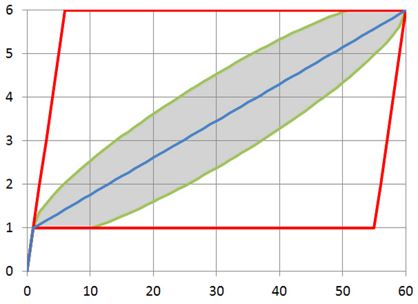
Thus, the statistical estimate conveys to us that the approximation of this function with a line segment is the correct idea.
In practice, of course, everything is usually more difficult than in theory. The following graph depicts the real distribution of key records in the Russian postal address directory, which contains over one million entries:
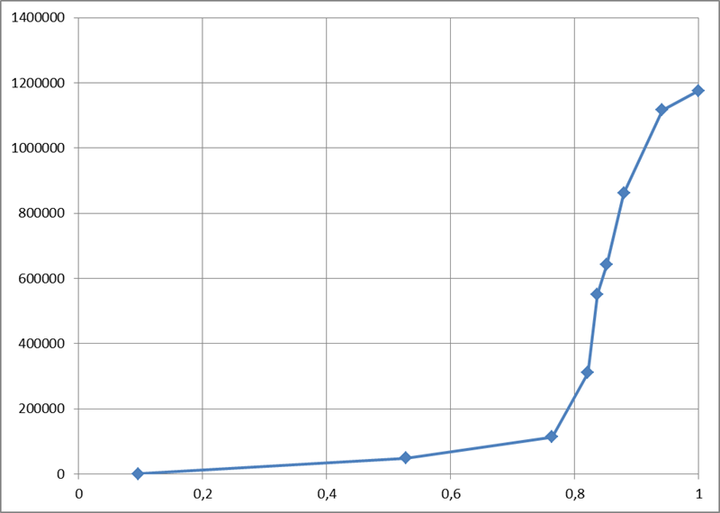
One look is sufficient to understand that while the function itself falls short of being a diagonal, calculating its values in just a few points and piecewise linear interpolation will provide us with an approximation of the function with the required accuracy. The approximation process converges very quickly along with an increase in the number of points: after all, each of the "pieces" of the function obeys the general properties, which means that it should lie within a small parallelogram and be largely located near this parallelogram’s diagonal.
Thus, we’ve arrived at the basic idea: instead of pumping out all the information from the entire table, it’s enough to calculate the relationship between the primary key and the record number at several points in the table, and, using piecewise interpolation, obtain a way to quickly jump to the record whose sequence number in the set approximately corresponds to the one specified.
The word "approximately" should not baffle us: after all, we are implementing a response to the action of the user setting the scrollbar knob. The user always does it "by sight": for example, having set it approximately in the middle, they expect to see records "from somewhere in the middle of the set," and certainly not the precise record with the number N/2, so it will be perfectly correct to resort to approximation.
Removing Simplifying Constraints
Now let’s remove the assumptions we’ve made earlier in order to simplify the articulation of the main idea.
-
First of all, we said that a unique key consists of one integer field. When a table has a compound key, and/or when the key contains not only integer values, but also strings, dates, etc., we can enumerate all possible combinations of key values so that they correspond to integers. The way to implement such numeration will be discussed later on in this article. The resulting numbers may be very large, but in general the task will be reduced to working with a single integer key. The bit length of such numbers must correspond to the cumulative size of the key fields, which is not surprising, because each number must unambiguously encode a field value. In Java, there is the
BigIntegerclass for working with integers of an arbitrary value, a class that allows you to perform all the required operations with huge numbers. -
Secondly, we assumed that the data is sorted by the primary key. But if we require sorting by another column, then we can mentally substitute this column at the top of the primary key column list. This won’t change anything: the uniqueness of primary key values is not violated by adding another column to it, but sorting by primary key will now mean sorting by this column and then by other primary key fields.
Thus, we can always reduce our task to mapping a table with a single integer key. Below we will consider the details of implementing this approach.
The main system components are displayed in the figure below:
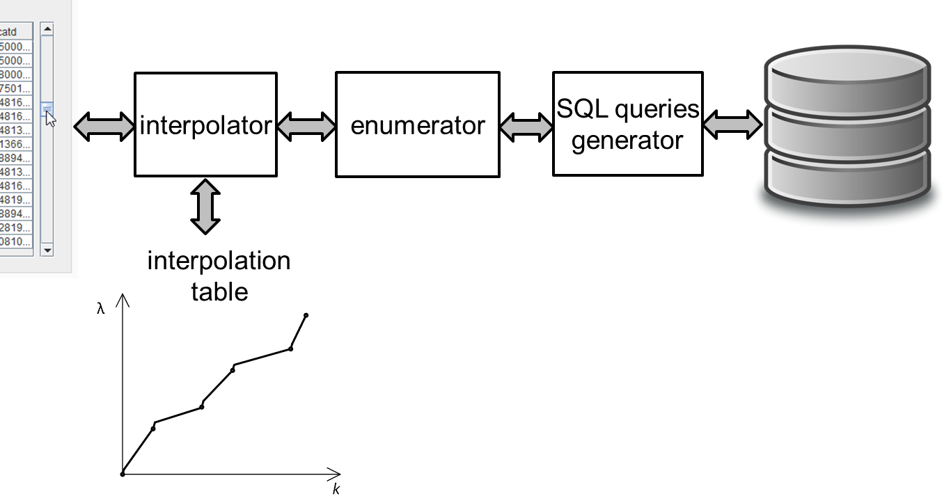
-
The interpolator holds a small table in memory and converts the knob position into the record’s sequence number and vice versa.
-
The enumerator converts the record’s sequence number to key field values.
-
The query generator creates
SELECT …queries to the database.
Step-By-Step Algorithm Operation: Scrolling
Let’s consider the example of the National Statistics Postcode Lookup (NSPL), which contains information on 1.75 million UK postal codes. The simplified structure of the directory is defined as follows:
CREATE TABLE nspl (
  postcode VARCHAR (7) NOT NULL PRIMARY KEY,
  area VARCHAR (60) NOT NULL,
  region VARCHAR (25) NOT NULL
);
CREATE INDEX ix_nspl ON nspl (area, postcode);
Let’s display this directory, sorting it by the name of the area and the postal code, imagining that the user scrolled approximately to the middle. Now let’s conduct a step-by-step analysis of this algorithm’s operation.
Step 1. We know the total number of records, and where the user placed the knob, thus, we can calculate the desired record number. Let’s say that this number is 657660.
Step 2. We can take the interpolation table and substitute the number of the desired record into it, performing an inverse interpolation. The output produced is the approximate sequence number of the key.
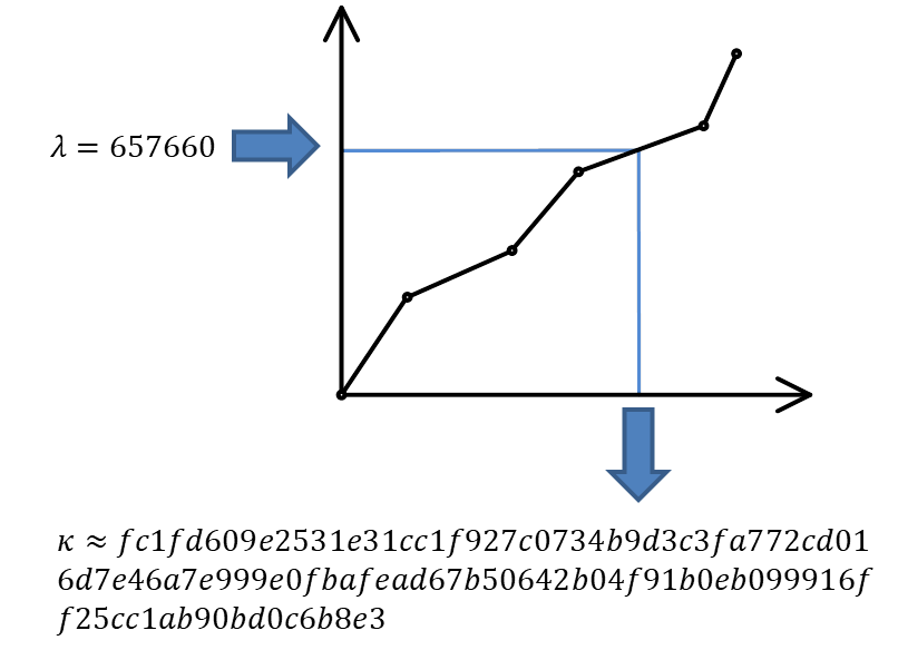
This is a huge number, which requires over a hundred characters even in the hexadecimal notation! For instance, as mentioned above, in Java the BigInteger class can be used to operate with this number.
Step 3. We’re moving on from the interpolator to the enumerator. The enumerator should calculate the key field values by the approximate sequence number of the key. Below we will discuss the way the enumerator works. For instance, it may produce a pair of the following values:
"area" -> "g\"\"oMsxr\"w2)-Mie(n6'.Njs9HSUR&4u4P9m9sWb&VDyS.v&p1i2\"w3X&OB "
"postcode" -> "L5&fxUR"
It looks like absolute gibberish made up of letters and symbols. In reality, it means only that, based on interpolation, the grid presumes that the record number 657660 should contain approximately this key field combination.
Step 4. Let’s insert the obtained fields in the following query:
SELECT ... FROM ... WHERE
  ("area", "postcode") >= (?, ?) LIMIT ...
A query of this kind, which uses the available composite index, will work instantly, finding the most suitable variant (area name, starting with the letter "g") in time O (log (N)):
"area" -> "Galgorm 1"
"postcode" -> "BT421AQ"
This and the following records are displayed to the user.
The first steps of the algorithm are just arithmetical operations, and the last step is a very effective SQL query, so the algorithm is executed very quickly. This allows to implement grid scrolling based on a table that contains almost 2 million records:
Suppose that the user has stopped scrolling the records and has not resumed scrolling for some time (i.e., 200 ms). This serves as a signal for our algorithm to begin the process of the knob position refinement. After all, we selected the record
"area" -> "Galgorm 1"
"postcode" -> "BT421AQ"
approximately in response to the request for the 657660th record. Its real position can be determined by executing the request
SELECT COUNT(*) FROM ... WHERE ("area", "postcode") < ('Galgorm 1', 'BT421AQ');This is a long-running query that loads the database. Thus, it is performed asynchronously, and only after it has been ascertained that the user has not been active for a while. The result of query execution is the exact position of the knob, which corresponds to the displayed data (in our case it turned out to be 686950).
Two things then will happen: 1) the knob in the user interface will "jump" to the refined position and 2) a new point will be added to the interpolation table, which will result in more accurate "guessing" of the values and smaller knob bounces next time.
Step-by-step Algorithm Operation: Positioning
Positioning is a task that works in reverse order. In this case, we know the primary key of the record, so we can instantly display the required rows of data to the user. The entire problem is the calculation of the knob position.
Let’s say we want to position a grid on a record with postcode W2 1UD.
Step 1. Let’s display the records corresponding to the user query. Since the primary key is known, this will be a quick operation for the database.
Step 2. Launch an asynchronous database query for the exact position of the knob (using the COUNT (*) query). This is a long-running operation, so we should not wait for its completion, and calculate and show the approximate knob position to the user while it is being executed.
Step 3. We will obtain the exact sequence number (a large integer) corresponding to the record
"area" -> "Westminster 015G"
"postcode" -> "W2  1UD"
Step 4. Insert the obtained number into the interpolation table and get the approximate number of the record: 1665834.
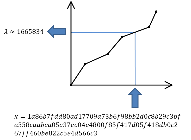
Step 5. Set the knob position of in accordance with this number, and return control to the user.
After some time, the query started in step 2 will be completed – in our case it returns the number 1670318. This will give us 1) the opportunity to add another point to the interpolation table; 2) if by that time the user has not scrolled through the records yet, we will specify the knob position.
Enumerator Operation
General Properties and Basic Cases
Now, only one question remains to be analyzed – how the enumerator works, converting the primary key values to large integers and back. The requirements for the numerating function are as follows:
-
The function is reversible. We should be able to calculate both the sequential number of the key value by key, and the key by its sequential number.
-
Generally, everything supported by the database as a key can act as an argument. This can be either a single value or a set of values (if the key is composite). The only operation possible with key values is comparison (in case of Java, you can say that the
Comparableinterface must implement the key data type). -
The function result type is
BigInteger. -
The order of numbers returned by the enumerator must match the order of the arguments from the point of view of the relational database. If you like math, then you can say that the function of the enumerator should postulate an isomorphism of the order.
How can this function be implemented?
For integer or Boolean values, the situation is trivial: these data types number themselves. Only trivial transformations are needed (0 – false, 1 – true, integers are reduced to a positive range). The timestamps are known to be reducible to a 64-bit integer value, so everything is also more or less clear in this regard.
Enumerator for Compound Keys
When ORDER BY X, Y sorting is used in a query, then at first the values of X are compared, and if they are equal, then the values of Y are also compared. This is the so-called lexicographic order. If it is known that the field Y can take only N values, then all possible combinations of X and Y values can be renumbered preserving the order, as shown in the figure below:
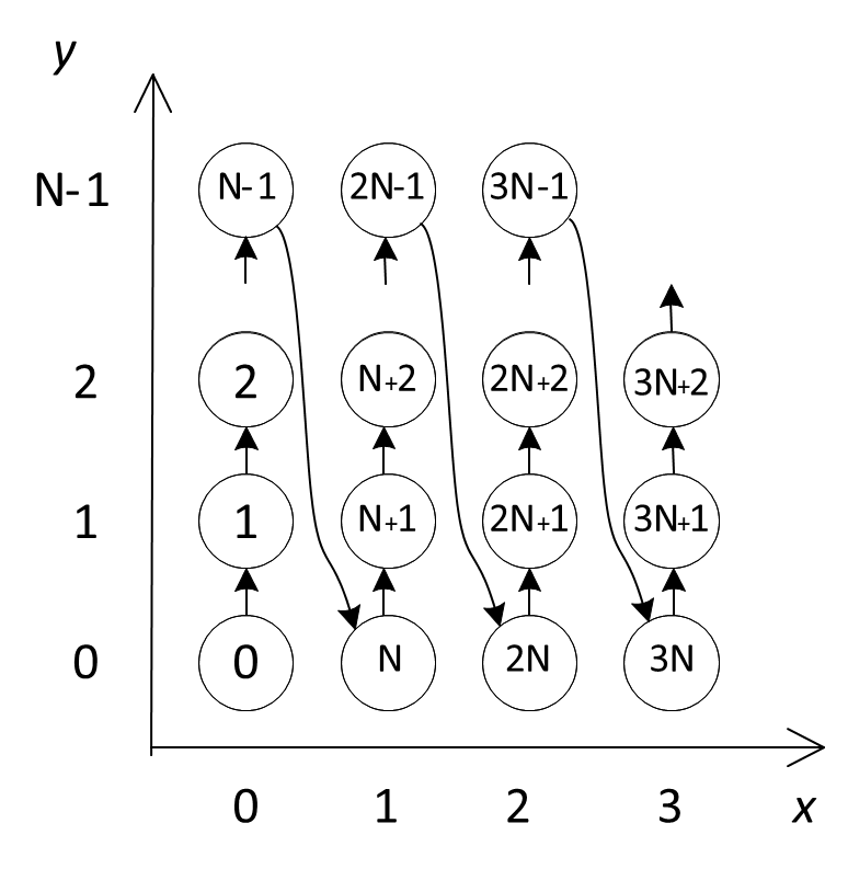
The formulas, using which we can calculate the enumerator’s direct and inverse function are trivial:
By "folding" the values of the composite key into a tree in direct calculation and "unfolding" the chain in reverse calculation, we can extrapolate this approach to a composite key with any number of fields, thereby resolving the task of creating a enumerator for a compound key of arbitrary length (if there are enumerators for each of the columns in the key).
Numbering for Strings
When the string length is unlimited, it becomes impossible to create the enumerator: for instance, in lexicographic order there are infinitely many strings 'aa', 'aaa', 'aaaa'… between 'a' and 'b', while there is always a finite number of integers between any two integers. A mathematician would say that the orders of the set of lexicographically ordered strings and the set of natural numbers are not isomorphic. Fortunately, in known RDBMS, an index can only be built on a limited-length string, which radically changes the case.
The number of strings no longer than symbols in an alphabet containing symbols is set by the formula
Indeed: we have one empty string, one-letter strings, two-letter strings, etc., up to . We can potentially include all these combinations in one list, and sort the list alphabetically.
Let’s imagine that we are operating only with the capital letters of the Latin alphabet and with strings no longer than four letters. Moreover, let us be concerned only with the segment of the alphabetically sorted list of all possible letter combinations between the words JOHN and MARY. Scrolling through this list is demonstrated in the following animation:
It is apparent that in the alphabetically ordered space of strings of no more than four characters in length, there are 45276 values between JOHN and MARY. All of them can be numbered and used to carry out amusing calculations, such as:
(3 * JOHN + MARY) / 4 = KEKC
(JOHN + MARY) / 2 = KUMT
(JOHN + 3 * MARY) / 4 = LKPI
and so on, which is exactly what we need to determine the most suitable primary keys corresponding to the user-selected knob positions.
Of course, all "real" names will have their own number (i.e., MARK = 45262).
A formula specifying the sequence number of a string of length in an alphabetically ordered space of strings of length not greater than m has the following form:
You can deduce it by induction. In fact:
-
an empty string (length 0) has number 0,
-
string
'A'(we are numbering all the letters in the alphabet from zero) has the length of 1 and number 1, -
string
'B'will have a number corresponding to the number of strings of length (between'A'and'B'there are all possible strings beginning with the letter'A'), therefore all single-letter strings have the number
and so on.
This formula can be calculated very fast if you prepare and cache the coefficients for in advance.
Computation of the inverse function also presents no difficulty: it is sufficient to perform a series of divisions with a remainder by the next coefficient, subtracting one at each step. Thus, symbol by symbol, the original string will be restored.
Conclusion
In order to simplify the presentation, I skipped the examination of a whole series of problems that arise in the practical implementation of an interpolation table-based grid. I will only list a few of them:
-
Collation rules. In fact, the rules that the database uses to compare strings are much more complicated than the usual lexicographic ordering. The real string-numbering algorithm must be modified so that it can take collation rules into account.
-
Working with
NULLvalues. As we know, some databases sortNULLvalues at the top of the list, and some — at the end. -
Cases where it is better for the grid to query rows from the table than to deal with interpolation.
-
Algorithms for the effective initial filling of the interpolation table.
-
Analysis of the interpolation quality. At what point is the interpolation table filled to a degree that no new points are required? In which cases does it make sense to reset the entire interpolation table or drop its individual points?
-
And a number of other small but significant details, the discussions of which would be enough for a separate story.
But I believe that the details examined here are sufficient to the understanding of the depths that this seemingly trivial task of displaying tabular data in the user interface conceals. It actually provides plenty of space for both mathematicians and software engineers to apply themselves.
You can read my articles on this topic in Russian here:
Or watch the videos of my presentations at JPoint 2017 and JUG.MSK meetup: